🏁 Determine offsides from any angle using the help of computer vision.
The Offside Detection in Soccer project is an advanced computer vision application that aims to accurately determine whether a player is in an offside position during a soccer match. Offside is a crucial rule in soccer, and its correct interpretation can significantly impact the outcome of a game. The project leverages the power of Python and various computer vision techniques to automate the offside decision-making process, reducing the reliance on human judgment and minimizing the potential for errors.
🔑 Key Features
Player Tracking
The project employs object detection and tracking algorithms to identify and track the positions of players on the field throughout the game.
The small circle represents each players furthest body part. This is the point that is used for determining offsides
Note: Referee and Goalie are ignored
💻 Code
For player tracking, we use YOLOv8's segmentation.
from yolo_segmentation import YOLOSegmentation

ys = YOLOSegmentation("yolov8m-seg.pt")
ret, frame = cap.read()

bboxes, classes, segmentations, scores = ys.detect(frame)
We used YOLOsegmentation rather than the default Object Detection so we can access the precise values for where the player is. This is used to detect which direction the player is facing which is used in our calculation for the Team Color Segmentation.
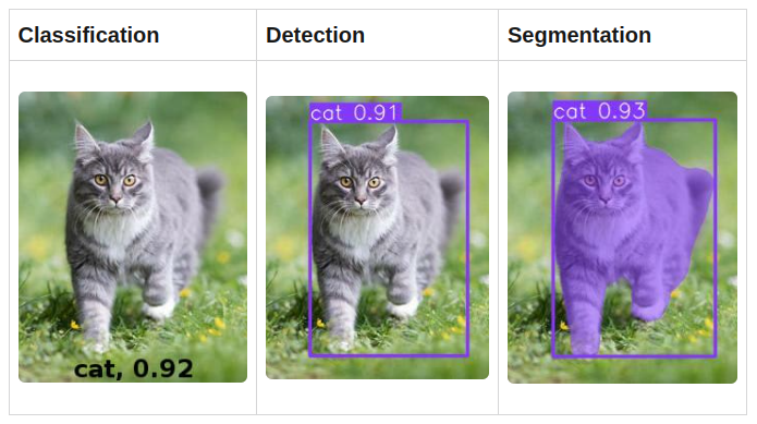
Image from freecodecamp.org
Then using OpenCV (cv2), we then draw the segmentation around each player using seg, an array of polygonal points.
import cv2

# Loop through each object detected
for index, (bbox, class_id, seg, score) in enumerate(zip(bboxes, classes, segmentations, scores)):
    # If object is a player (class 0)
    if class_id == 0:
        cv2.polylines(frame, [seg], True, (0,255,255), 3)
Team Color Classification
The system also analyzes the colors of the player jerseys to distinguish between teams. By detecting the dominant colors on the players' uniforms, the algorithm can categorize them into teams.
- Uses bounding box to determine which way the player is facing
- Creates a smaller box at the most likely spot of the player's jersey
- Gets the average color in the smaller box
- Uses euclidean distance to group players into 3 groups: team1, team2, and team3 (referees and goalkeepers)
The smaller square represents the box used to determine the jersey color.
💻 Code
Determining what team each player was on was more complex than we initially thought. Our solution was to create a smaller box around where we expect the player's main jersey color to be most dominant.
Because the bounding box surrounds the entirety of the player, we can't expect the player to always be in the center. So we determine which way a player is facing. To do this we calculated the distances from the head to the farthest X values.
# First we find the farthest left and right
minX = min(seg, key=itemgetter(0))[0]
maxX = max(seg, key=itemgetter(0))[0]
# And bottom value
maxY = max(seg, key=itemgetter(1))[1]

# Then we determine the distance from the top corner
# of the head to the maximum value
distLeft = int(abs(seg[0][0] - minX))
distRight = int(abs(seg[0][0] - maxX))
Then we created a smaller box, compared the distances, and shifted the box appropriately.
# Create smaller box points around player for detecting color
newX = int((x2 - x)/3 + x)
newY = int((y2 - y)/5 + y)
newX2 = int(2*(x2 - x)/3 + x)
newY2 = int(2*(y2 - y)/5 + y)

# Shift new box based on player orientation
if(distRight > distLeft):
    # Shift left
    newX = int(newX - ((distRight)/distLeft)/1.5)
    newX2 = int(newX2 - ((distRight)/distLeft)/1.5)
else:
    # Shift right
    newX = int(newX + ((distLeft)/distRight)*1.5)
    newX2 = int(newX2 + ((distLeft)/distRight)*1.5)
Now we have:
Before
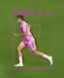 After
After
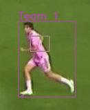
Now, we get the average color inside the box. We can pass in the smaller box and average each pixel inside of it.
def get_average_color(a):
    avg_color = np.mean(a, axis=(0,1))
    return avg_color
To classify each team, we first calculate the euclidean distance from each average color to the team colors. This is essentially plotting the two bgr values as xyz points on a 3-dimentional graph. Then we calculate the distance between those two points.
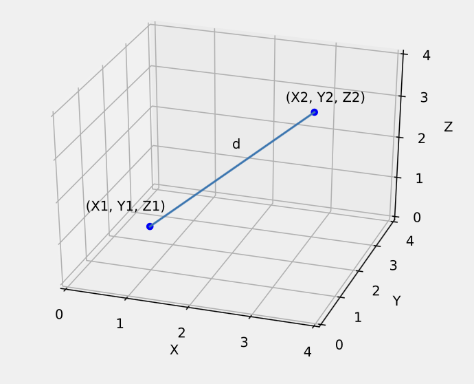
We use that value to classify the colors into different teams. By doing this for each player, each player is now assigned a team.
def assign_custom_label(color, team1_bgr, team2_bgr):

    # Define the threshold distance for outliers
    threshold_distance = 120.0  # Adjust this value as needed based on the color space

    # Calculate the distance to team1 and team2 colors
    team1_distance = euclidean_distance(color, team1_bgr)
    team2_distance = euclidean_distance(color, team2_bgr)

    # Check if the color is too far from both team2 and team1
    if team1_distance > threshold_distance and team2_distance > threshold_distance:
        # For referees, goalkeepers, and non-players
        return "group3"
    elif team1_distance < team2_distance:
        return "group1"
    else:
        return "group2"
Perspective Transform onto 2D Map
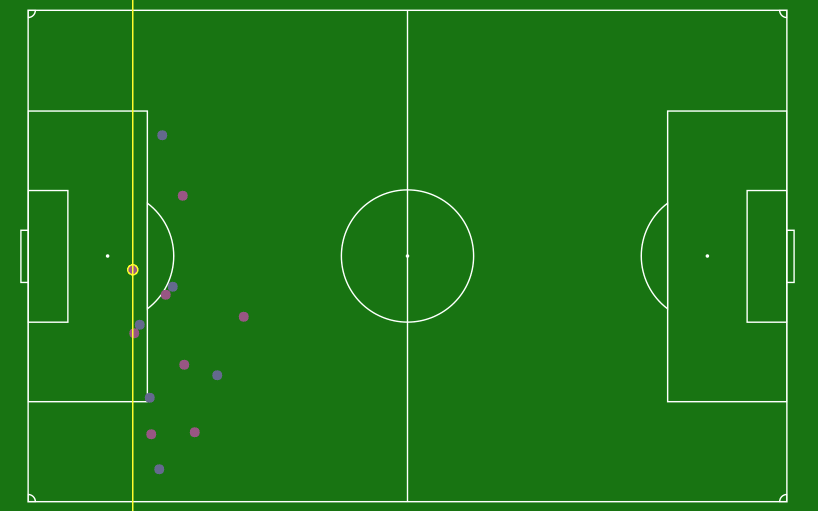
The most important part of this project is implementing perspective transform to get information on the actual distance down the field players are. This information is crucial for making offside determinations.
- Uses OpenCV's perspective transform
- Passes in each players furthest positioning (including any head, body, and feet) and places it on a 2D map of the field
- Determines who is nearest to the goal line and highlights that player
The red dots represents the points used for transforming the perspective.
💻 Code
To transform a 3D images onto a 2D plane we used OpenCV's function getPerspectiveTransform() and perspectiveTransform().
By feeding in 8 corresponding points (4 original and 4 new), we can transform our players on the 3D field onto our 2D field by passing in each player's coordinate.
# pts1 are 4 original points and pts2 are 4 new points
M = cv2.getPerspectiveTransform(pts1,pts2)

# pts3 is our point we want to transform
pts3o = cv2.perspectiveTransform(pts3[None, :, :], M)
x = int(pts3o[0][0][0])
y = int(pts3o[0][0][1])

# New point on the 2d image
new_p = (x,y)
To determine who is the last player, we append all 2D points to a list called new_points and determine who has the minimum X value.
max_point_X, max_point_Y = min(new_points, key=itemgetter(0))[0], min(new_points, key=itemgetter(0))[1]Draw a line at that point and we can see who the last player is.
🪴 Areas of Improvement
- Reliability: The project could always have higher accuracy and reliability in offside decisions. It is only as accurate as the points it is given for perspective transform.
- Real-Time Video Analysis: The system would be more useful if it could process live video feeds from soccer matches, enabling real-time offside detection during gameplay.
- Pitch Detection: If the system could automatically detect and classify points on the field, the process would be entirely automated. This is a limitation created by non-fixed camera angles and could be solved with a fixed view of the field.
- Deep Sort: If players could be tracked throughout the game, we could implement automatic statistics on the amount of time spent offside.
🚀 Further Uses
- Team Formation Analysis: The project can further analyze the players' positions to determine the formation of each team during a particular play. This information can be valuable for understanding the dynamics of the game and how the offside decision impacts team strategies.
- Player Jersey Number Recognition: The system could utilize Optical Character Recognition (OCR) techniques to read the jersey numbers of players on the field. This allows the identification of individual players and track their movement and time spent offside.
💻 Technology
- OpenCV
- NumPy
- YoloV8